How to automate measurements with Python
As a system and application engineer, I’ve saved countless hours by automating measurements with software such as LabVIEW. Although I’ve used it to build measurement applications, I’ve started to replace LabVIEW with Python for basic lab measurements where I don’t need develop an easy-to-use GUI for others to use. When I just need to quickly take some measurements, Python lets me save them in an easy-to-read format and plot them.
To understand why, let’s look at the main advantages of Python and discuss a working example of a Python application. The best way to convey the convenience and power of Python is to describe a complete, working Python automation script, such as the one I used to automate the measurement of a VR’s (voltage regulator’s) load-regulation curve (load regulation is the variation of the output voltage as the output current – the load – increases).
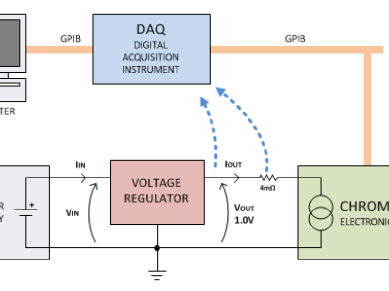
VRs are divided into two categories: zero-droop regulators and droop regulators. Zero-droop regulators have zero output resistance; the output-voltage setpoint shouldn’t change with increasing output currents. On the contrary, droop regulators are said to have a ‘loadline’, which means they’re designed to have a specific equivalent output resistance. The regulator used for this example has a zero-current output voltage of 1 V and a programmed loadline of 2.5 mΩ. Figure 1 shows the test setup.

Figure 1. The VR under test connects to an electronic load while a DAQ system measures the output current through a shunt resistor.
The load current (the VR output current) is applied using a Chroma 63201 electronic load. The output current is measured by acquiring the voltage across a calibrated 4-mΩ shunt resistor. Both voltage and current are acquired using a Keysight 34970A DAQ (data-acquisition system), and both the DAQ and the electronic load communicate to a computer over a GPIB link. The goal of our measurement is to verify that the output voltage is within specification across a range of output currents; Figure 2 shows the application’s flowchart.

Figure 2. The application sets the electronic load, measures the VR output voltage and current, and saves the results.
The next pages describe the code I used to make these measurements. There, you’ll find links to download the code as a text file.
Basic code structure
Below, you can find the first part of the automation script code listing. In Python, comments are preceded by #:
[Download all code from this article as a text file.]
import numpy as np # 1
import pandas as pd # 2
import visa, time # 3
chroma = visa.instrument(‘GPIB::2’) # 4
daq = visa.instrument(‘GPIB::9’) # 5
results = pd.DataFrame() # 6
loads = np.arange(0,20+2,2) # 7
for load in loads: # 8
# Measure the current and the voltage
# Save the results
Lines 1 to 3 import libraries that contain methods used later in the code:
Numpy is a package used for scientific computing. In this example, Numpy is used to generate the array of output-current values.
Pandas (a library for data manipulation and analysis) creates a very powerful data structure to store the results of our measurements.
Visa is the PyVISA library that we use to control our instruments.
Time is a handy library that we need to generate some time delays.
Note that the imported Numpy and Pandas libraries have been renamed to np and pd to keep the code clean. All the libraries mentioned in this article are either already available with your Python distribution, or they can be easily installed from online repositories.
Lines 4 to 5 create the objects that we will use to access the Chroma electronic load and the Keysight DAQ. This is where PyVISA comes into play: all we need to do is to call the instrument method and provide a string to indicate the GPIB address of the instruments on the bus.
Line 6 creates the results dataframe to store the measurement results. A dataframe is a two-dimensional labeled data structure with columns of potentially different data types. Using a dataframe instead of an array will allow us to reference to columns using an easy-to-remember string instead of number, and to mix numbers and text in the data itself.
Line 7 creates an array of real numbers from 0 to 20 with a step of 2. These numbers will represent the values of the output current in amps at which we want to measure VOUT.
Line 8 is used to construct the “for” loop. Note that the syntax is very easy to understand: every time the loop is executed a variable called load will be generated with a value equal to a new element of the loads array. The loop ends when all the elements of the array have been used. It is interesting to highlight how Python uses indentation to define code hierarchy, without relying on any type of parenthesis. This is very useful because it keeps the code clean and legible.
Now that we have the defined our main for loop, we need to talk to the instruments to program the current, then read the voltage, and save the results.
Talking to instruments saving data, and plotting
Look at the second part of the code:
[Download all code from this article as a text file.]
for load in loads: # 8
chroma.write(‘CURR:STAT:L1 %.2f’ % load) # 9
chroma.write(‘LOAD ON’) # 10
time.sleep(1) # 11
temp = {} # 12
daq.write(‘MEAS:VOLT:DC? AUTO,DEF,(@101)’) # 13
temp[‘Vout’] = float(daq.read()) # 14
daq.write(‘MEAS:VOLT:DC? AUTO,DEF,(@102)’) # 15
temp[‘Iout’] = float(daq.read())/0.004 # 16
results = results.append(temp, ignore_index=True) # 17
print “%.2fA\t%.3fV” % (temp[‘Iout’],temp[‘Vout’]) # 18
chroma.write(‘LOAD OFF’) # 19
results.to_csv(‘Results.csv’) # 20
Lines 9 to 10 configure the desired load current and turn the load on. Communicating with instruments over GPIB is all about using read/write methods and knowing the command strings the instrument accepts as indicated in the instrument manual. Similar to other programming languages, %.2f is a placeholder that is replaced at run-time with the content of the variable load. It also indicates that we want the data to be represented as a real number with two decimal digits. Line 11 generates a one-second delay, useful to make sure the instruments and the circuits have reached a steady-state condition.
Line 12 generates an empty object (called dictionary in Python) that we use to temporarily store the results of one iteration of the loop.
Lines 13 to 16 are used to measure the output voltage and current. The first command tells the instrument what we want to do (measure DC voltage with automatic scale) and the desired acquisition channel. The output voltage and current are acquired on channel 101 and 102, respectively. The second command reads the result back and stores it into temp. The data is returned as a string, so it must be converted to a real number using the float function. Also, because the DAQ is measuring voltages, we need to divide the reading by the shunt resistance (0.004 Ω) to get the correct value for the current.
Note how easy it is to save data in an organized fashion using Python and Pandas: the fields of the temp dictionary don’t need to be defined in advance and are accessed using meaningful strings. There’s no need to remember the relationship between column number and data as we would have to do if we had instead decided to use an array to store the data.
In line 17 we append the dictionary to the results dataframe. Note that results doesn’t need to be initialized as well; every time a new line is appended, any new field will be added to the dataframe.
Line 18 is optional, but it can be useful to print the present voltage and current on the terminal, in particular for long measurements, as a way to make sure the application is still running and to know how far along it is.
In lines 19 to 20 the load is turned off and the data is saved on disk. For the latter, each dataframe object has a handy embedded method to save the data on a CSV file.
The power of dataframes
To explore the power of using Python and Pandas dataframes, just add this code between line 16 and line 17.
temp[‘Vout_id’] = 1.0 – 2.5e-3*temp[‘Iout’] # A
temp[‘Vout_err’] = temp[‘Vout_id’] – temp[‘Vout’] # B
temp[‘Pass’] = ‘Yes’ # C
if (abs(temp[‘Vout_err’]) > temp[‘Vout_id’]*0.001): # D
temp[‘Pass’] = ‘No’ # E
Lines A and B generate two new fields of the dataframe. Vout_id contains the ideal DC setpoint value of the output voltage given the measured current and the ideal zero-current setpoint (1 V) and loadline. Vout_err is the absolute error between the ideal and measured voltage.
Lines D and E add the Pass field to the dataframe. The content of the field is a string indicating whether a hypothetic specification of ±0.1% on the output-voltage accuracy is met or not. In Figure 3, you can see how the saved CSV file looks in Excel. It’s marvelous: numeric data and text are in the same table, and even column headers are automatically generated from the names of the dataframe fields.

Figure 3. The Python script can save data in CSV format, which easily opens in Excel.
Data analysis and plotting with Pyplot
The snippet of code described in the previous section allowed us to determine whether the output voltage was within the “tolerance band” around its ideal value. Another interesting piece of information we might want to get out of this experiment is the exact value of the loadline, which is the slope of the VOUT-vs-IOUT curve. If you don’t remember how to do a linear fit of the acquired data, don’t worry, for Python has a function for it, too. Just insert this code at the end of script:
from scipy.stats import linregress # A
loadline = linregress(results[‘Iout’], results[‘Vout’]) # B
print “The loadline is %.2f mohm” % (loadline[0]*1000) # C
print “The intercept point is %.3f V” % loadline[1] # D
Line A imports a single method from Scipy’s Stats module. In line B, we feed the imported linregress method with the X and Y coordinates of the points we are trying to fit. Finally, we print the result on the terminal in lines C and D. Linregress returns several results organized in an array, with the slope saved at index 0 and the intercept point at index 1. Other information available are the correlation coefficient and the standard error of the estimate.
With such a small dataset (20 points) it is possible to use Excel to generate plots. A three-line example show how that can be done in Python: just add them at the end of the script described previously (the ro parameter of the plot method indicates that I wanted to use red circle markers):
import matplotlib.pyplot as plt # A
plt.plot(results[‘Iout’],results[‘Vout’], ‘ro’) # B
plt.show() # C
Pyplot is a module of the Python’s Matplotlib library that contains plenty of methods to plot graphs. Better still, the methods have been designed to be almost identical to MATLAB’s. You can see the results of these three lines of code in Figure 4. The window and the graphics are automatically generated by Pyplot, and they appear “out of thin air” from the terminal window.

Figure 4. Pyplot lets you plot data, which eliminates having to open the data in Excel.
Python is an excellent choice to automate your laboratory setup and avoid tedious hours of measurements because it is simple to use, easy to understand, and extremely flexible and powerful. LabVIEW is, however, still the king of the GUI. In general, I think LabVIEW is better suited for applications requiring a nice graphical interface and that aren’t required to execute complex loops or data processing. For instance, I still use LabVIEW to design most of the applications that are customer-facing and so need to be pretty but are rarely complicated. For all the other applications and automation needs, though, Python is now my first choice.
What is Python and why use it?
Python is an interpreted, object-oriented, high-level programming language with dynamic semantic. Since its first release in 1991, Python has grown in popularity and it is now used in a wide range of applications; it is one of the most commonly taught programming languages in major universities and online courses. What makes Python such a great “first” programming language are its simplicity and easy-to-learn syntax and readability (some say “it is written in plain English”), all combined with great versatility and capabilities.
Don’t think that Python is “just” a good teaching or academic language with little or no professional applications. On the contrary, Python is used heavily in web applications and data analysis by many top organizations such as Google, Yahoo and NASA. It is a very attractive language for rapid application development and it can be used to automate complex electronic instruments and make data collection more efficient.
Python’s advantages are not limited to its ease of use. Python scripts can be run cross-platform on any major operative system, as long as the free Python interpreter is installed. Python is also extremely powerful and is extensively used for data analysis and complex mathematical calculations.
Why consider Python for laboratory automation? Most of the test setups I implement are quite simple: 95% of the time the task involves measuring one or more signals (such as voltage, current, or temperature) at different times, or over a set of values of another independent variable. Implementing this requires little more than looping through your independent variable, acquiring the signals, and finally saving the data for further analysis. It is really simple to do this in Python, thanks to its straightforward, no-nonsense grammar and its useful, handy libraries.
In addition, a Python script is very easy to modify. If you later decide you want to acquire your signals over two independent variables instead of one, all you need to do is to nest the loop you had designed before inside another loop. This might require only a handful of new lines of code. Thanks to Python’s high legibility, you can easily change scripts written by other people as well (something I always dreaded to do with LabVIEW applications).
A programming language has a definite edge over graphical languages as the complexity increases. Python is excellent at math and data analysis and it is used by data scientists to extract trends from gigantic, complex data sets. Many people are used to relying on MATLAB for complex data analysis. As a matter of fact, Python is also an excellent (and free) replacement for MATLAB, thanks to its many MATLAB-compatible libraries (as shown in the example at the end of the article). I often prefer Python over Excel for plotting graphs too, unless the graphs are really simple and the dataset is small. If you are interested in using Python for data analysis, I recommend Python for Data Analysis by Wes McKinney or enrolling in the free online course Intro to Data Science on Udacity.
If you’ve ever used a programming language, you likely didn’t have any problem following me until this point, but you may be wondering how Python communicate with measurement instruments. Not to worry, as there is a library for that, too: PyVISA is an easy-to-use package that connects Python scripts to GPIB, RS232, USB, and Ethernet instruments.
LabVIEW is still the best option to make applications with user friendly GUIs. The process is not as straightforward with Python, but it is not very difficult either. My GUI toolkit of choice is usually PyQT. If you are interested in knowing more about this topic, see Rapid GUI Programming with Python and QT by Mark Summerfield.
If you want to learn Python, I recommend enrolling in a Massive Open Online Course (MOOC) such as Udacity, Coursera or Udemy. Introductory programming courses are usually free of charge and taught by some of the best engineers and teachers in the field. Python has a very minimal setup and shallow learning curve, so you will be able to write useful applications in less than a day.
Mac and Linux users will find Python already available in the terminal and only need to install a few additional libraries using a package management system such as pip. For Windows users, I recommend installing Python(x,y), which contains a scientific-oriented Python distribution with all the libraries you can possibly need in a single package. I usually also install IPython, a command shell that enables interactive computing in Python and makes developing new applications even easier.
About the author
Fabrizio Guerrieri is a Full-Stack Electrical Engineer with experience from IC design to coding and product marketing. Currently Guerrieri is a Sr. System/Application Engineer at Maxim Integrated working on isolated DC-DC regulators and Battery Management Systems. Before Maxim, Guerrieri managed a team of Application Engineers at Volterra Semiconductor, invented of the world’s first Single-Photon Counting Camera and worked on quantum imaging at MIT. Guerrieri has a PhD in EE from Politecnico di Milano.
 If you enjoyed this article, you will like the following ones: don't miss them by subscribing to :